Analyzing simulation data from HOOMD-blue at runtime#
The following script shows how to use freud to compute the radial distribution function \(g(r)\) on data generated by the molecular dynamics simulation engine HOOMD-blue during a simulation run.
Generally, most users will want to run analyses as post-processing steps, on the saved frames of a particle trajectory file. However, it is possible to use analysis callbacks in HOOMD-blue to compute and log quantities at runtime, too. By using analysis methods at runtime, it is possible to stop a simulation early or change the simulation parameters dynamically according to the analysis results.
HOOMD-blue can be installed with conda install -c conda-forge hoomd.
The simulation script runs a Monte Carlo simulation of spheres, with outputs parsed with numpy.genfromtxt.
[1]:
%matplotlib inline
import freud
import hoomd
import matplotlib.pyplot as plt
import numpy as np
from hoomd import hpmc
[2]:
hoomd.context.initialize("")
system = hoomd.init.create_lattice(hoomd.lattice.sc(a=1), n=10)
mc = hpmc.integrate.sphere(seed=42, d=0.1, a=0.1)
mc.shape_param.set("A", diameter=0.5)
rdf = freud.density.RDF(bins=50, r_max=4)
w6 = freud.order.Steinhardt(l=6, wl=True)
def calc_rdf(timestep):
hoomd.util.quiet_status()
snap = system.take_snapshot()
hoomd.util.unquiet_status()
rdf.compute(system=snap, reset=False)
def calc_W6(timestep):
hoomd.util.quiet_status()
snap = system.take_snapshot()
hoomd.util.unquiet_status()
w6.compute(system=snap, neighbors={"num_neighbors": 12})
return np.mean(w6.particle_order)
# Equilibrate the system a bit before accumulating the RDF.
hoomd.run(1e4)
hoomd.analyze.callback(calc_rdf, period=100)
logger = hoomd.analyze.log(
filename="output.log",
quantities=["w6"],
period=100,
header_prefix="#",
overwrite=True,
)
logger.register_callback("w6", calc_W6)
hoomd.run(1e4)
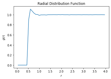
# Store the computed RDF in a file
np.savetxt(
"rdf.csv", np.vstack((rdf.bin_centers, rdf.rdf)).T, delimiter=",", header="r, g(r)"
)
HOOMD-blue v2.7.0-77-g568406147 DOUBLE HPMC_MIXED MPI TBB SSE SSE2 SSE3 SSE4_1 SSE4_2 AVX AVX2
Compiled: 10/28/2019
Copyright (c) 2009-2019 The Regents of the University of Michigan.
-----
You are using HOOMD-blue. Please cite the following:
* J A Anderson, C D Lorenz, and A Travesset. "General purpose molecular dynamics
  simulations fully implemented on graphics processing units", Journal of
  Computational Physics 227 (2008) 5342--5359
* J Glaser, T D Nguyen, J A Anderson, P Liu, F Spiga, J A Millan, D C Morse, and
  S C Glotzer. "Strong scaling of general-purpose molecular dynamics simulations
  on GPUs", Computer Physics Communications 192 (2015) 97--107
-----
-----
You are using HPMC. Please cite the following:
* J A Anderson, M E Irrgang, and S C Glotzer. "Scalable Metropolis Monte Carlo
  for simulation of hard shapes", Computer Physics Communications 204 (2016) 21
  --30
-----
HOOMD-blue is running on the CPU
notice(2): Group "all" created containing 1000 particles
** starting run **
Time 00:00:10 | Step 3878 / 10000 | TPS 387.761 | ETA 00:00:15
Time 00:00:20 | Step 7808 / 10000 | TPS 392.99 | ETA 00:00:05
Time 00:00:25 | Step 10000 / 10000 | TPS 398.521 | ETA 00:00:00
Average TPS: 392.122
---------
notice(2): -- HPMC stats:
notice(2): Average translate acceptance: 0.933106
notice(2): Trial moves per second:        1.56844e+06
notice(2): Overlap checks per second:     4.07539e+07
notice(2): Overlap checks per trial move: 25.9838
notice(2): Number of overlap errors:      0
** run complete **
** starting run **
Time 00:00:35 | Step 13501 / 20000 | TPS 349.776 | ETA 00:00:18
Time 00:00:45 | Step 17001 / 20000 | TPS 349.699 | ETA 00:00:08
Time 00:00:54 | Step 20000 / 20000 | TPS 352.224 | ETA 00:00:00
Average TPS: 350.471
---------
notice(2): -- HPMC stats:
notice(2): Average translate acceptance: 0.932846
notice(2): Trial moves per second:        1.40185e+06
notice(2): Overlap checks per second:     3.63552e+07
notice(2): Overlap checks per trial move: 25.9338
notice(2): Number of overlap errors:      0
** run complete **
[3]:
rdf_data = np.genfromtxt("rdf.csv", delimiter=",")
plt.plot(rdf_data[:, 0], rdf_data[:, 1])
plt.title("Radial Distribution Function")
plt.xlabel("$r$")
plt.ylabel("$g(r)$")
plt.show()
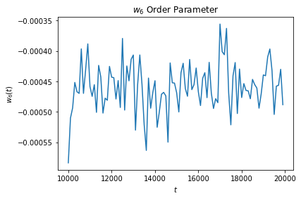
[4]:
w6_data = np.genfromtxt("output.log")
plt.plot(w6_data[:, 0], w6_data[:, 1])
plt.title("$w_6$ Order Parameter")
plt.xlabel("$t$")
plt.ylabel("$w_6(t)$")
plt.show()