Density Module
Overview
Computes the complex pairwise correlation function. |
|
Computes the density of a system on a grid. |
|
Computes the local density around a particle. |
|
Computes the RDF \(g \left( r \right)\) for supplied data. |
Details
The freud.density module contains various classes relating to the
density of the system. These functions allow evaluation of particle
distributions with respect to other particles.
-
class
freud.density.CorrelationFunction¶ Bases:
freud.locality._SpatialHistogram1DComputes the complex pairwise correlation function.
The correlation function is given by \(C(r) = \left\langle s^*_1(0) \cdot s_2(r) \right\rangle\) between two sets of points \(p_1\) (
points) and \(p_2\) (query_points) with associated values \(s_1\) (values) and \(s_2\) (query_values). Computing the correlation function results in an array of the expected (average) product of all values at a given radial distance \(r\).The values of \(r\) where the correlation function is computed are controlled by the
r_maxanddrparameters to the constructor.r_maxdetermines the maximum distance at which to compute the correlation function anddris the step size for each bin.Note
Self-correlation: It is often the case that we wish to compute the correlation function of a set of points with itself. If
query_pointsis the same aspoints, not provided, orNone, we omit accumulating the self-correlation value in the first bin.- Parameters
bins (unsigned int) – The number of bins in the RDF.
r_max (float) – Maximum pointwise distance to include in the calculation.
-
bin_centers¶ The centers of each bin in the histogram.
- Type
\((N_{bins}, )\)
numpy.ndarray
-
property
bin_counts¶ The bin counts in the histogram.
- Type
-
bin_edges¶ The edges of each bin in the histogram. Is one element larger becauseeach bin has a lower and upper bound.
- Type
\((N_{bins}+1, )\)
numpy.ndarray
-
property
box¶ The box object used in the last computation.
- Type
-
compute¶ Calculates the correlation function and adds to the current histogram.
- Parameters
system – Any object that is a valid argument to
freud.locality.NeighborQuery.from_system.values ((\(N_{points}\))
numpy.ndarray) – Values associated with the system points used to calculate the correlation function.query_points ((\(N_{query\_points}\), 3)
numpy.ndarray, optional) – Query points used to calculate the correlation function. Uses the system’s points ifNone(Default value =None).query_values ((\(N_{query\_points}\))
numpy.ndarray, optional) – Query values used to calculate the correlation function. UsesvaluesifNone. (Default value =None).neighbors (
freud.locality.NeighborListor dict, optional) – Either aNeighborListof neighbor pairs to use in the calculation, or a dictionary of query arguments (Default value: None).reset (bool) – Whether to erase the previously computed values before adding the new computation; if False, will accumulate data (Default value: True).
-
property
correlation¶ Expected (average) product of all values at a given radial distance.
- Type
(\(N_{bins}\))
numpy.ndarray
-
default_query_args¶ The default query arguments are
{'mode': 'ball', 'r_max': self.r_max}.
-
plot¶ Plot complex correlation function.
- Parameters
ax (
matplotlib.axes.Axes, optional) – Axis to plot on. IfNone, make a new figure and axis. (Default value =None)- Returns
Axis with the plot.
- Return type
-
class
freud.density.GaussianDensity¶ Bases:
freud.util._ComputeComputes the density of a system on a grid.
Replaces particle positions with a Gaussian blur and calculates the contribution from each to the proscribed grid based upon the distance of the grid cell from the center of the Gaussian. The resulting data is a regular grid of particle densities that can be used in standard algorithms requiring evenly spaced point, such as Fast Fourier Transforms. The dimensions of the image (grid) are set in the constructor, and can either be set equally for all dimensions or for each dimension independently.
- Parameters
-
property
box¶ Box used in the calculation.
- Type
-
compute¶ Calculates the Gaussian blur for the specified points.
- Parameters
system – Any object that is a valid argument to
freud.locality.NeighborQuery.from_system.
-
property
density¶ The image grid with the Gaussian density.
- Type
(\(w_x\), \(w_y\), \(w_z\))
numpy.ndarray
-
plot¶ Plot Gaussian Density.
- Parameters
ax (
matplotlib.axes.Axes, optional) – Axis to plot on. IfNone, make a new figure and axis. (Default value =None)- Returns
Axis with the plot.
- Return type
-
class
freud.density.LocalDensity¶ Bases:
freud.locality._PairComputeComputes the local density around a particle.
The density of the local environment is computed and averaged for a given set of query points in a sea of data points. Providing the same points calculates them against themselves. Computing the local density results in an array listing the value of the local density around each query point. Also available is the number of neighbors for each query point, giving the user the ability to count the number of particles in that region. Note that the computed density is essentially a number density (that allows for fractional values as described below). If your particles have a specific volume, you can compute a volume density by simply multiplying the output by the volume of the particles.
In order to provide sufficiently smooth data, data points can be fractionally counted towards the density. Rather than perform compute-intensive area (volume) overlap calculations to determine the exact amount of overlap area (volume), the LocalDensity class performs a simple linear interpolation relative to the centers of the data points. Specifically, a point is counted as one neighbor of a given query point if it is entirely contained within the
r_max, half of a neighbor if the distance to its center is exactlyr_max, and zero if its center is a distance greater than or equal tor_max + diameterfrom the query point’s center. Graphically, this looks like: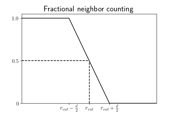
- Parameters
-
property
box¶ Box used in the calculation.
- Type
-
compute¶ Calculates the local density for the specified points.
- Parameters
system – Any object that is a valid argument to
freud.locality.NeighborQuery.from_system.query_points ((\(N_{query\_points}\), 3)
numpy.ndarray, optional) – Query points used to calculate the correlation function. Uses the system’s points ifNone(Default value =None).neighbors (
freud.locality.NeighborListor dict, optional) –Either a
NeighborListof neighbor pairs to use in the calculation, or a dictionary of query arguments (Default value: None).
-
default_query_args¶ The default query arguments are
{'mode': 'ball', 'r_max': self.r_max + 0.5*self.diameter}.
-
property
density¶ Density of points per query point.
- Type
(\(N_{points}\))
numpy.ndarray
-
property
num_neighbors¶ Number of neighbor points for each query point.
- Type
(\(N_{points}\))
numpy.ndarray
-
class
freud.density.RDF¶ Bases:
freud.locality._SpatialHistogram1DComputes the RDF \(g \left( r \right)\) for supplied data.
Note that the RDF is defined strictly according to the pair correlation function, i.e.
\[g(r) = V\frac{N-1}{N} \langle \delta(r) \rangle\]In the thermodynamic limit, the fraction tends to unity and the limiting behavior of \(\lim_{r \to \infty} g(r)=1\) is recovered. However, for very small systems the long range behavior of the radial distribution will instead tend to \(\frac{N-1}{N}\). If you are analyzing a very small system but wish to recover the more familiar behavior, you may use the normalize flag to enforce this requirement upon construction of this object. Note that this will have little to no effect on larger systems (for example, for systems of 100 particles the RDF will differ by 1%).
Note
2D:
freud.density.RDFproperly handles 2D boxes. The points must be passed in as[x, y, 0].- Parameters
bins (unsigned int) – The number of bins in the RDF.
r_max (float) – Maximum interparticle distance to include in the calculation.
r_min (float, optional) – Minimum interparticle distance to include in the calculation (Default value =
0).normalize (bool, optional) – Scale the RDF values by \(\frac{N_{query\_points}+1}{N_{query\_points}+1}\). This argument primarily exists to deal with standard RDF calculations where no special
query_pointsorneighborsare provided, but where the number ofquery_pointsis small enough that the long-ranged limit of \(g(r)\) deviates significantly from \(1\). It should not be used ifquery_pointsis provided as a different set of points, or if unusual query arguments are provided tocompute(), specifically if :code`exclude_ii` is set toFalse. This normalization is not meaningful in such cases and will simply convolute the data.
-
bin_centers¶ The centers of each bin in the histogram.
- Type
\((N_{bins}, )\)
numpy.ndarray
-
property
bin_counts¶ The bin counts in the histogram.
- Type
-
bin_edges¶ The edges of each bin in the histogram. Is one element larger becauseeach bin has a lower and upper bound.
- Type
\((N_{bins}+1, )\)
numpy.ndarray
-
property
box¶ The box object used in the last computation.
- Type
-
compute¶ Calculates the RDF and adds to the current RDF histogram.
- Parameters
system – Any object that is a valid argument to
freud.locality.NeighborQuery.from_system.query_points ((\(N_{query\_points}\), 3)
numpy.ndarray, optional) – Query points used to calculate the RDF. Uses the system’s points ifNone(Default value =None).neighbors (
freud.locality.NeighborListor dict, optional) –Either a
NeighborListof neighbor pairs to use in the calculation, or a dictionary of query arguments (Default value: None).reset (bool) – Whether to erase the previously computed values before adding the new computation; if False, will accumulate data (Default value: True).
-
default_query_args¶ The default query arguments are
{'mode': 'ball', 'r_max': self.r_max}.
-
property
n_r¶ Histogram of cumulative bin_counts values. More precisely,
n_r[i]is the average number of points contained within a ball of radiusR[i]+dr/2centered at a givenquery_pointaveraged over allquery_pointsin the last call tocompute().- Type
(\(N_{bins}\),)
numpy.ndarray
-
plot¶ Plot radial distribution function.
- Parameters
ax (
matplotlib.axes.Axes, optional) – Axis to plot on. IfNone, make a new figure and axis. (Default value =None)- Returns
Axis with the plot.
- Return type
-
property
rdf¶ Histogram of RDF values.
- Type
(\(N_{bins}\),)
numpy.ndarray