BondOrder

Computing Bond Order Diagrams

The freud.environment module analyzes the local environments of particles. In this example, the freud.environment.BondOrder class is used to plot the bond order diagram (BOD) of a system of particles.

import numpy as np
import freud
import matplotlib.pyplot as plt
import matplotlib
from mpl_toolkits.mplot3d import Axes3D
import util

Setup

Our sample data will be taken from an face-centered cubic (FCC) structure. The array of points is rather large, so that the plots are smooth. Smaller systems may need to use accumulate to gather data from multiple frames in order to smooth the resulting array’s statistics.

box, points = util.make_fcc(nx=40, ny=40, nz=40, noise=0.1)
orientations = np.array([[1, 0, 0, 0]]*len(points))

Now we create a BondOrder compute object and create some arrays useful for plotting.

rmax = 3 # This is intentionally large
n_bins_theta = 100
n_bins_phi = 100
k = 0 # This parameter is ignored
n = 12 # Chosen for FCC structure
bod = freud.environment.BondOrder(rmax=rmax, k=k, n=n, n_bins_t=n_bins_theta, n_bins_p=n_bins_phi)

phi = np.linspace(0, np.pi, n_bins_phi)
theta = np.linspace(0, 2*np.pi, n_bins_theta)
phi, theta = np.meshgrid(phi, theta)
x = np.sin(phi) * np.cos(theta)
y = np.sin(phi) * np.sin(theta)
z = np.cos(phi)

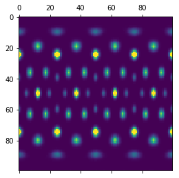
Computing the Bond Order Diagram

Next, we use the compute method and the bond_order property to return the array. Note that we use freud’s method chaining here, where a compute method returns the compute object.

bod_array = bod.compute(box=box, ref_points=points, ref_orientations=orientations, points=points, orientations=orientations).bond_order
bod_array = np.clip(bod_array, 0, np.percentile(bod_array, 99)) # This cleans up bad bins for plotting
plt.matshow(bod_array)
plt.show()

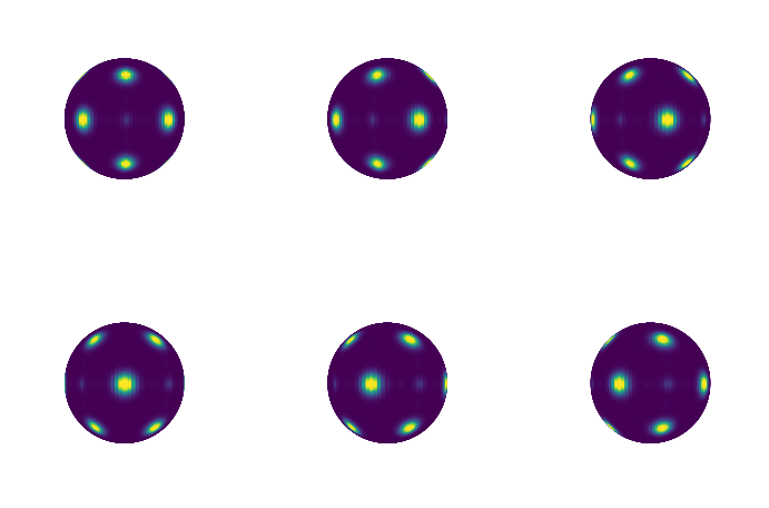
Plotting on a sphere

This code shows the bond order diagram on a sphere as the sphere is rotated. The code takes a few seconds to run, so be patient.

fig = plt.figure(figsize=(12, 8))
for plot_num in range(6):
    ax = fig.add_subplot(231 + plot_num, projection='3d')
    ax.plot_surface(x, y, z, rstride=1, cstride=1, shade=False,
                    facecolors=matplotlib.cm.viridis(bod_array.T / np.max(bod_array)))
    ax.set_xlim(-1, 1)
    ax.set_ylim(-1, 1)
    ax.set_zlim(-1, 1)
    ax.set_axis_off()
    # View angles in degrees
    view_angle = 0, plot_num*15
    ax.view_init(*view_angle)
plt.show()

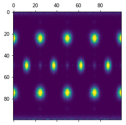
Using Neighbor Lists

We can also construct neighbor lists and use those to determine bonds instead of the rmax and n values in the BondOrder constructor. For example, we can filter for a range of bond lengths. Below, we only consider neighbors between \(r_{min} = 2.5\) and \(r_{max} = 3\) and plot the resulting bond order diagram.

lc = freud.locality.LinkCell(box=box, cell_width=3)
nlist = lc.compute(box, points, points).nlist
nlist.filter_r(box, points, points, rmax=3, rmin=2.5)
bod_array = bod.compute(box=box, ref_points=points, ref_orientations=orientations,
                        points=points, orientations=orientations, nlist=nlist).bond_order
bod_array = np.clip(bod_array, 0, np.percentile(bod_array, 99)) # This cleans up bad bins for plotting
plt.matshow(bod_array)
plt.show()