Analyzing simulation data from HOOMD-blue at runtime
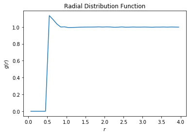
The following script shows how to use freud to compute the radial distribution function \(g(r)\) on data generated by the molecular dynamics simulation engine HOOMD-blue during a simulation run.
Generally, most users will want to run analyses as *post-processing* steps, on the saved frames of a particle trajectory file. However, it is possible to use analysis callbacks in HOOMD-blue to compute and log quantities at runtime, too. By using analysis methods at runtime, it is possible to stop a simulation early or change the simulation parameters dynamically according to the analysis results.
HOOMD-blue can be installed with conda install -c conda-forge hoomd.
The simulation script runs a Monte Carlo simulation of spheres, with outputs parsed with numpy.genfromtxt.
[1]:
%matplotlib inline
import hoomd
from hoomd import hpmc
import freud
import numpy as np
import matplotlib.pyplot as plt
[2]:
hoomd.context.initialize('')
system = hoomd.init.create_lattice(
    hoomd.lattice.sc(a=1), n=10)
mc = hpmc.integrate.sphere(seed=42, d=0.1, a=0.1)
mc.shape_param.set('A', diameter=0.5)

rdf = freud.density.RDF(rmax=4, dr=0.1)

box = freud.box.Box.from_box(system.box)
w6 = freud.order.LocalWlNear(box, 4, 6, 12)

def calc_rdf(timestep):
    hoomd.util.quiet_status()
    snap = system.take_snapshot()
    hoomd.util.unquiet_status()
    rdf.accumulate(box, snap.particles.position)

def calc_W6(timestep):
    hoomd.util.quiet_status()
    snap = system.take_snapshot()
    hoomd.util.unquiet_status()
    w6.compute(snap.particles.position)
    return np.mean(np.real(w6.Wl))

# Equilibrate the system a bit before accumulating the RDF.
hoomd.run(1e4)
hoomd.analyze.callback(calc_rdf, period=100)

logger = hoomd.analyze.log(filename='output.log',
                           quantities=['w6'],
                           period=100,
                           header_prefix='#',
                           overwrite=True)

logger.register_callback('w6', calc_W6)

hoomd.run(1e4)

# Store the computed RDF in a file
np.savetxt('rdf.csv', np.vstack((rdf.R, rdf.RDF)).T,
           delimiter=',', header='r, rdf')
HOOMD-blue v2.6.0-7-g60513d253 DOUBLE HPMC_MIXED MPI TBB SSE SSE2 SSE3 SSE4_1 SSE4_2 AVX AVX2
Compiled: 06/11/2019
Copyright (c) 2009-2019 The Regents of the University of Michigan.
-----
You are using HOOMD-blue. Please cite the following:
* J A Anderson, C D Lorenz, and A Travesset. "General purpose molecular dynamics
  simulations fully implemented on graphics processing units", Journal of
  Computational Physics 227 (2008) 5342--5359
* J Glaser, T D Nguyen, J A Anderson, P Liu, F Spiga, J A Millan, D C Morse, and
  S C Glotzer. "Strong scaling of general-purpose molecular dynamics simulations
  on GPUs", Computer Physics Communications 192 (2015) 97--107
-----
-----
You are using HPMC. Please cite the following:
* J A Anderson, M E Irrgang, and S C Glotzer. "Scalable Metropolis Monte Carlo
  for simulation of hard shapes", Computer Physics Communications 204 (2016) 21
  --30
-----
HOOMD-blue is running on the CPU
notice(2): Group "all" created containing 1000 particles
** starting run **
Time 00:00:10 | Step 3869 / 10000 | TPS 386.859 | ETA 00:00:15
Time 00:00:20 | Step 7834 / 10000 | TPS 396.436 | ETA 00:00:05
Time 00:00:25 | Step 10000 / 10000 | TPS 386.636 | ETA 00:00:00
Average TPS: 390.536
---------
notice(2): -- HPMC stats:
notice(2): Average translate acceptance: 0.933106
notice(2): Trial moves per second:        1.56207e+06
notice(2): Overlap checks per second:     4.05885e+07
notice(2): Overlap checks per trial move: 25.9838
notice(2): Number of overlap errors:      0
** run complete **
** starting run **
Time 00:00:35 | Step 13151 / 20000 | TPS 315.038 | ETA 00:00:21
Time 00:00:45 | Step 16301 / 20000 | TPS 314.415 | ETA 00:00:11
Time 00:00:55 | Step 19519 / 20000 | TPS 321.741 | ETA 00:00:01
Time 00:00:57 | Step 20000 / 20000 | TPS 329.027 | ETA 00:00:00
Average TPS: 317.613
---------
notice(2): -- HPMC stats:
notice(2): Average translate acceptance: 0.932846
notice(2): Trial moves per second:        1.2704e+06
notice(2): Overlap checks per second:     3.29464e+07
notice(2): Overlap checks per trial move: 25.9338
notice(2): Number of overlap errors:      0
** run complete **
[3]:
rdf_data = np.genfromtxt('rdf.csv', delimiter=',')
plt.plot(rdf_data[:, 0], rdf_data[:, 1])
plt.title('Radial Distribution Function')
plt.xlabel('$r$')
plt.ylabel('$g(r)$')
plt.show()
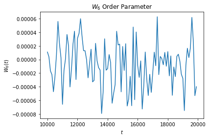
[4]:
w6_data = np.genfromtxt('output.log')
plt.plot(w6_data[:, 0], w6_data[:, 1])
plt.title('$W_6$ Order Parameter')
plt.xlabel('$t$')
plt.ylabel('$W_6(t)$')
plt.show()