Voronoi
The voronoi module finds the Voronoi diagram of a set of points, while respecting periodic boundary conditions (which are not handled by scipy.spatial.Voronoi, documentation). This is handled by replicating the points using periodic images that lie outside the box, up to a specified buffer distance.
This case is two-dimensional (with z=0 for all particles) for simplicity, but the voronoi module works for both 2D and 3D simulations.
[1]:
import numpy as np
import freud
import matplotlib
import matplotlib.pyplot as plt
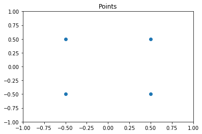
First, we generate some sample points.
[2]:
points = np.array([
    [-0.5, -0.5],
    [0.5, -0.5],
    [-0.5, 0.5],
    [0.5, 0.5]])
plt.scatter(points[:,0], points[:,1])
plt.title('Points')
plt.xlim((-1, 1))
plt.ylim((-1, 1))
plt.show()

# We must add a z=0 component to this array for freud
points = np.hstack((points, np.zeros((points.shape[0], 1))))
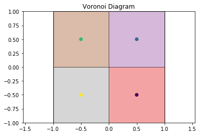
Now we create a box and a voronoi compute object. Note that the buffer distance must be large enough to ensure that the points are duplicated sufficiently far outside the box for the qhull algorithm. Results are only guaranteed to be correct when the buffer is large enough: buffer \(>= L/2\), for the longest box side length \(L\).
[3]:
L = 2
box = freud.box.Box.square(L)
voro = freud.voronoi.Voronoi(box, L/2)
Next, we use the compute method to determine the Voronoi polytopes (cells) and the polytopes property to return their coordinates. Note that we use freud’s method chaining here, where a compute method returns the compute object.
[4]:
cells = voro.compute(box=box, positions=points).polytopes
print(cells)
[array([[ 0., -1.,  0.],
       [-1., -1.,  0.],
       [-1.,  0.,  0.],
       [ 0.,  0.,  0.]]), array([[ 0., -1.,  0.],
       [ 0.,  0.,  0.],
       [ 1.,  0.,  0.],
       [ 1., -1.,  0.]]), array([[-1.,  0.,  0.],
       [ 0.,  0.,  0.],
       [ 0.,  1.,  0.],
       [-1.,  1.,  0.]]), array([[0., 0., 0.],
       [0., 1., 0.],
       [1., 1., 0.],
       [1., 0., 0.]])]
We create a helper function to draw the Voronoi polygons using matplotlib.
[5]:
def draw_voronoi(box, points, cells, nlist=None, color_by_sides=False):
    ax = plt.gca()
    # Draw Voronoi cells
    patches = [plt.Polygon(cell[:, :2]) for cell in cells]
    patch_collection = matplotlib.collections.PatchCollection(patches, edgecolors='black', alpha=0.4)
    cmap = plt.cm.Set1

    if color_by_sides:
        colors = [len(cell) for cell in voro.polytopes]
    else:
        colors = np.random.permutation(np.arange(len(patches)))

    cmap = plt.cm.get_cmap('Set1', np.unique(colors).size)
    bounds = np.array(range(min(colors), max(colors)+2))

    patch_collection.set_array(np.array(colors))
    patch_collection.set_cmap(cmap)
    patch_collection.set_clim(bounds[0], bounds[-1])
    ax.add_collection(patch_collection)

    # Draw points
    plt.scatter(points[:,0], points[:,1], c=colors)
    plt.title('Voronoi Diagram')
    plt.xlim((-box.Lx/2, box.Lx/2))
    plt.ylim((-box.Ly/2, box.Ly/2))

    # Set equal aspect and draw box
    ax.set_aspect('equal', 'datalim')
    box_patch = plt.Rectangle([-box.Lx/2, -box.Ly/2], box.Lx, box.Ly, alpha=1, fill=None)
    ax.add_patch(box_patch)

    # Draw neighbor lines
    if nlist is not None:
        bonds = np.asarray([points[j] - points[i] for i, j in zip(nlist.index_i, nlist.index_j)])
        box.wrap(bonds)
        line_data = np.asarray([[points[nlist.index_i[i]],
                                 points[nlist.index_i[i]]+bonds[i]] for i in range(len(nlist.index_i))])
        line_data = line_data[:, :, :2]
        line_collection = matplotlib.collections.LineCollection(line_data, alpha=0.3)
        ax.add_collection(line_collection)

    # Show colorbar for number of sides
    if color_by_sides:
        cb = plt.colorbar(patch_collection, ax=ax, ticks=bounds, boundaries=bounds)
        cb.set_ticks(cb.formatter.locs + 0.5)
        cb.set_ticklabels((cb.formatter.locs - 0.5).astype('int'))
        cb.set_label("Number of sides", fontsize=12)
    plt.show()
Now we can draw the Voronoi diagram from the example above.
[6]:
draw_voronoi(box, points, voro.polytopes)
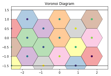
This also works for more complex cases, such as this hexagonal lattice.
[7]:
def hexagonal_lattice(rows=3, cols=3, noise=0):
    # Assemble a hexagonal lattice
    points = []
    for row in range(rows*2):
        for col in range(cols):
            x = (col + (0.5 * (row % 2)))*np.sqrt(3)
            y = row*0.5
            points.append((x, y, 0))
    points = np.asarray(points)
    points += np.random.multivariate_normal(mean=np.zeros(3), cov=np.eye(3)*noise, size=points.shape[0])
    # Set z=0 again for all points after adding Gaussian noise
    points[:, 2] = 0

    # Wrap the points into the box
    box = freud.box.Box(Lx=cols*np.sqrt(3), Ly=rows, is2D=True)
    points = box.wrap(points)
    return box, points

# Compute the Voronoi diagram and plot
box, points = hexagonal_lattice()
voro = freud.voronoi.Voronoi(box, np.max(box.L)/2)
voro.compute(box=box, positions=points)
draw_voronoi(box, points, voro.polytopes)
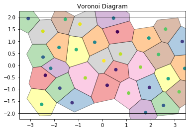
For noisy data, we see that the Voronoi diagram can change substantially. We perturb the positions with 2D Gaussian noise:
[8]:
box, points = hexagonal_lattice(rows=4, cols=4, noise=0.04)
voro = freud.voronoi.Voronoi(box, np.max(box.L)/2)
voro.compute(box=box, positions=points)
draw_voronoi(box, points, voro.polytopes)
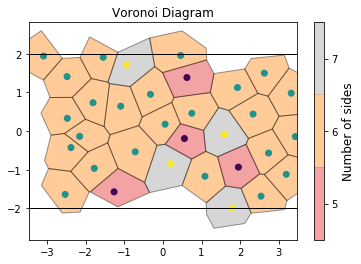
If we color by the number of sides of each Voronoi cell, we can see patterns in the defects: 5-gons and 7-gons tend to pair up.
[9]:
draw_voronoi(box, points, voro.polytopes, color_by_sides=True)
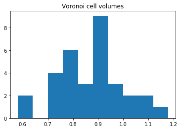
We can also compute the volumes of the Voronoi cells. Here, we plot them as a histogram:
[10]:
voro.computeVolumes()
plt.hist(voro.volumes)
plt.title('Voronoi cell volumes')
plt.show()
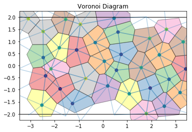
The voronoi module also provides freud.locality.NeighborList objects, where particles are neighbors if they share an edge in the Voronoi diagram. The NeighborList effectively represents the bonds in the Delaunay triangulation.
[11]:
voro.computeNeighbors(box=box, positions=points)
nlist = voro.nlist
draw_voronoi(box, points, voro.polytopes, nlist=nlist)
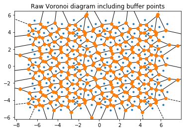
The voronoi property stores the raw scipy.spatial.qhull.Voronoi object from scipy.
Important: The plots below also show the replicated buffer points, not just the ones inside the periodic box. freud.voronoi is intended for use with periodic systems while scipy.spatial.Voronoi does not recognize periodic boundaries.
[12]:
print(type(voro.voronoi))
from scipy.spatial import voronoi_plot_2d
voronoi_plot_2d(voro.voronoi)
plt.title('Raw Voronoi diagram including buffer points')
plt.show()
<class 'scipy.spatial.qhull.Voronoi'>